Naive Path Tracing: From Formula to Code
Naive Path Tracing: From Formula to Code
위 포스팅은 아래와 같은 자료들을 참고하였습니다.
- Rendering: Next Event Estimation: https://www.cg.tuwien.ac.at/sites/default/files/course/4411/attachments/08_next%20event%20estimation.pdf
- CSE 168 - Computer Graphics II-Rendering(UCSD)
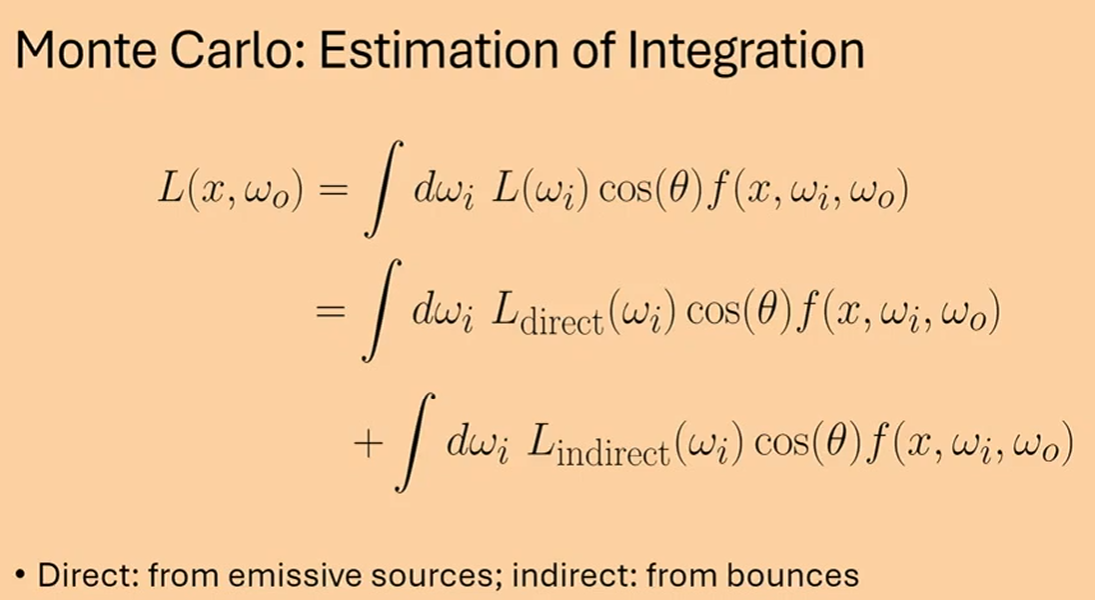
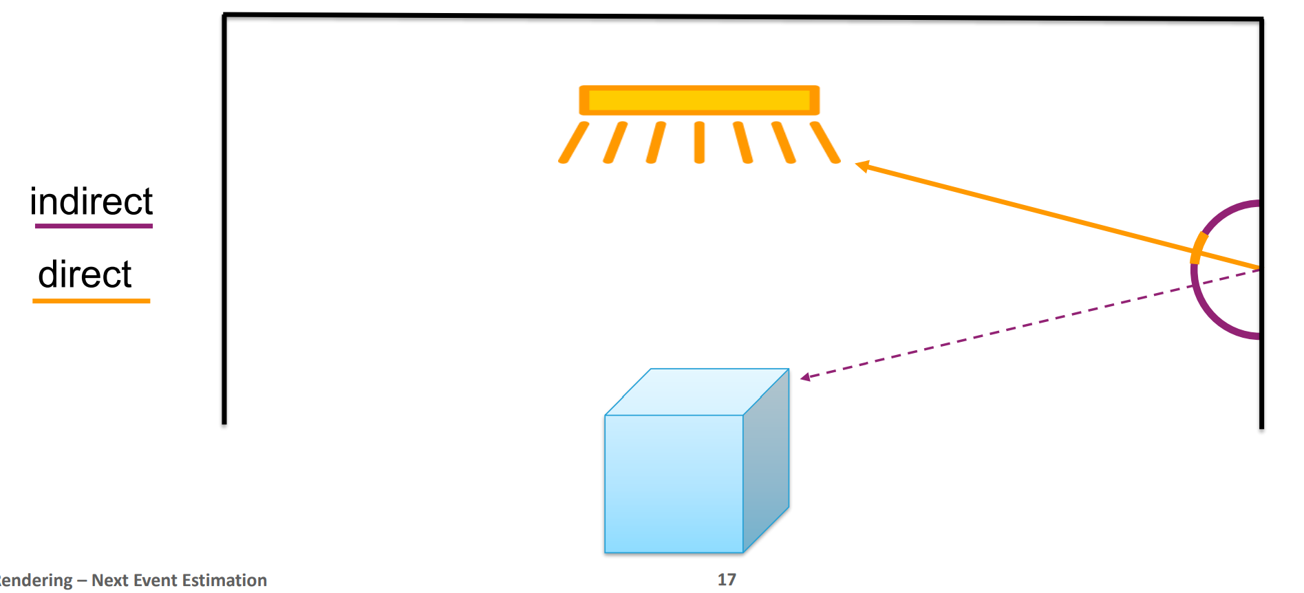
우린 Naive한 Monte Carlo 시뮬레이션의 식은 크게 두 가지로 이루어져있다는 것을 알 수 있다. 바로, direct와 indirect라는 것이다.
Direct Lighting
Direct Lighting은 NEE 기법을 이용할 것이다. Next Event Estimation이란 Direct Lighting 항에 대해서 낮은 분산으로 계산하기 위한 방법이다. 일종의 Direct Lighting 검사기+계산기인 것이다.
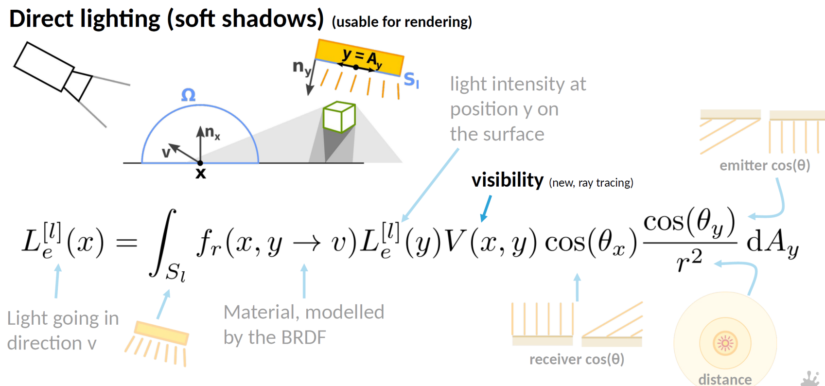
그래서 위의 그림을 보면, 화면에서 발사한 광선이 물체와 교차되면 해당 지점을 hit으로 두고 광원으로 부터 균등 샘플링한다. 그렇게 추출한 표면과 hit을 이용해 표면→광원까지의 벡터인 dir_to_light(wi) 을 구한다. 그러면 우리는 들어오는 빛($w_i$)의 방향을 알아낸 것이다. 계산에 필요한 $cos\theta_i$를 구하기 위해서, $\vec{n}\cdot\vec{w_i}$를 이용한다.
- BRDF 함수 $f_r$: 빛이 들어온 방향(입사조도)과 나가는 방향(방사조도)을 통해서 (들어오고 나가는)변환율
- $L_i$: 표면 $x$에 들어오는 빛의 양
- $cos\theta_i$: 빛이 들어온 방향($w_i$)에 따라서, 실제로 표면 $x$에 맞는 빛의 세기
그러면 $cos\theta_o$는 어떻게 구할까? 결국 광원 입장에서는 표면(hit)→광원의 벡터인 $w_i$의 반대부호인 $-w_i$가 결국 $w_o$이 된다. 최종적으로 광원 샘플링할 때 사용하였던, $\vec{light_n}$과 $w_o$를 dot product하여 $cos\theta_o$를 구할 수 있다.
            // 라이트 표면 균등 샘플
            double r1 = 2.0 * PI * rng.uniform();
            double z = 1.0 - 2.0 * rng.uniform();            // in [-1,1]
            double rxy = std::sqrt(std::max(0.0, 1.0 - z * z));
            // Light의 normal vector를 균등 샘플링을 통해 추출한다.
            Vec3 light_n = normalize(Vec3(rxy * std::cos(r1), rxy * std::sin(r1), z));
            Vec3 x_light = light.p + light_n * light.r;

            // 방향/거리/코사인
            Vec3 dir_to_light = x_light - hit;
            double d2 = dot(dir_to_light, dir_to_light);
            double d = std::sqrt(d2);
            Vec3  wi = dir_to_light / d; // normalize
            double cos_i = std::max(0.0, dot(nl, wi));   // 표면 쪽
            double cos_l = std::max(0.0, dot(light_n, -1.0 * wi)); // 라이트 쪽
$G$를 구하기 위한 재료들을 모두 모았다. $V(x, x’)$함수의 경우에는 visibility term으로써, 광원과 물체사이 가로막는 물체가 있는지 체크하는 항이다.
                // PPT의 pdf_solid_angle
                double area = 4.0 * PI * light.r * light.r;         // 구의 표면적 공식
                double pdf_omega = (d2) / (cos_l * area);           // 표면균등 샘플의 고체각 pdf
                pdf_omega /= static_cast<double>(lights.size());

                Vec3 f = obj.albedo * (1.0 / PI);                  // Lambert f
                Vec3 Li = light.e;

                Vec3 contrib = f * Li * cos_i / pdf_omega; // 여기서, cos_i / pdf_omega = G / pdf_solid_angle
                result.direct += contrib;
최종적으로 contrib 라는 변수를 통해 G를 구하게 된다. pdf_omega 라는 항에 $cos\theta_o$와 $area$를 이용하는 것을 알 수 있는데, 이것은 jacobian을 기반으로 한 것이다.
- 자코비안 참고 내용
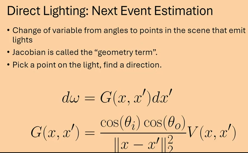
- 적분을 수행하는 단위는 $d\omega_i$이다. 여기서, 이것이 의미하는 것은 반구가 가리키는 면적을 의미한다. 그러면, Direct Lighting이니 굳이 반구의 면적을 적분할 필요는 없고 우리는 평면을 통해서 적분 값을 구해도 된다. 이걸 좀 더 수학적으로 ‘방향을 기반으로 된 적분 → 표면을 기반으로 한 적분’으로 바꾸는 것이다.
- 여기서, 사용되는 개념이 Jacobian인데, ‘반구의 각도→ 광원 표면 면적’으로 투영시킨 것이다. 그러면, 또 하나 의문이 생기는 것은 ‘왜 $cos\theta_o$가 등장하는 것인가?’ 평면으로 투영된 곳의 면적은 원래 넓이에서 $|\vec{n} \cdot \vec{\omega}|$를 곱한 값이어야 하기 때문이다. \(dω=\frac{dA_{proj}}{r^2}=\frac{cosθ_o}{r^2}dA(x^′)\)
Indirect Lighting
Direct Lighting을 구하는 방법은 알았으니, Indirect Lighting은 어떻게 구하는 것인지 살펴보자. 먼저, Indirect Lighting은 기본적으로 재귀를 통해서 값을 계산해 나간다. 하지만, 코드적으로 무한에 가깝게 재귀를 들어가는 것은 비용적으로 너무 비싼 계산이다. 그렇기 때문에 반복문을 통해서 ‘몇 번 튕길지’를 하이퍼 파라미터로써 설정하여 제한한다.
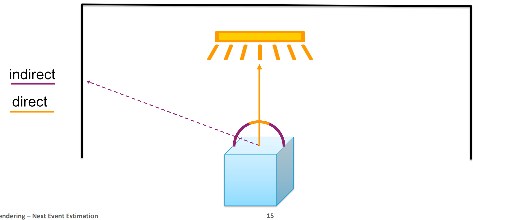
노랑색과 같은 광선은 NEE을 통해서 계산하고 그 다음 튕긴 광선은 indirect 계산을 수행해야한다. 다만 이 PPT의 이미지에서 주의할 점은 광선의 시작은 무조건 ‘유저가 보는 화면’이라는 것이다. 그러니까, 위 PPT의 기본적인 전제는 ‘화면에서 발사한 광선이 PPT에서 가리키는 포인트에 맞은 후의 상황’이라는 것이다.
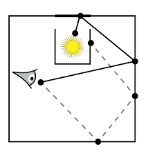
위 이미지와 같이, Indirect 란, 화면에서 발사한 광선이 이리 튕기고 저리 튕겨서 최종적으로 광원에 도달하게 되는 경우가 Indirect Lighting이라고 할 수 있는 것이다. 그 이외의 광선은 화면에 영향을 줄 수 없으니 계산하지 않게 된다.
Bounce of Ray
        // ----- Indirect bounce (cosine-weighted hemisphere) -----
        double r1 = 2.0 * PI * rng.uniform(); // φ = 2 * PI * u
        double r2 = rng.uniform();
        double r2s = std::sqrt(r2);

        Vec3 u = normalize(cross((std::fabs(nl.x) > 0.1 ? Vec3(0, 1, 0) : Vec3(1, 0, 0)), nl));
        Vec3 v = cross(nl, u);
        Vec3 d = normalize(u * (std::cos(r1) * r2s)   // u·(cosφ·sinθ)
							        + v * (std::sin(r1) * r2s)      // v·(sinφ·sinθ)
							        + nl * std::sqrt(1.0 - r2));    // w·cosθ, cosθ=√(1-ξ)

        ray = Ray(hit + nl * 1e-4, d);
        beta *= obj.albedo;  // for cosine-weighted sampling of Lambertian: f*cos/pdf = albedo
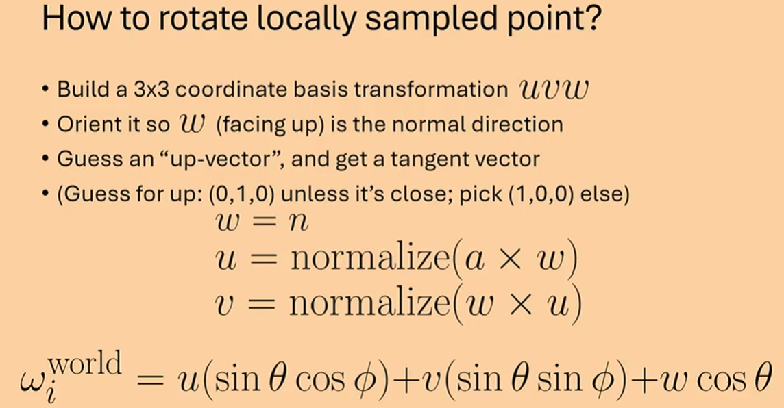
아까 이야기했듯이, 광선이 물체와 만나게 되면 튕겨야한다. 이때 어디로 튕길지에 대한 정의를 반구범위로 정의하게 되는데, 위 코드가 반구 범위로 샘플링하는 수식을 코드화시킨 결과이다.
a 는 up 벡터의 후보를 의미한다. normal vector와 거의 평행한 경우를 피하기 위해 (0, 1, 0)과 (1, 0, 0) 둘 중에 선택하는 것이다. $sin\theta$ 대신에 r2s 라는 변수가 사용된다. 해당 이유는 균등 반구 샘플링이 아닌 코사인 가중 샘플링을 위함이다.
샘플의 분포가 코사인 값에 비례하도록 $\theta$를 추출하는 과정을 한번 살펴보자. 우리는 이것을 알기위해서 역변환 샘플링을 사용하게 된다. CDF를 풀면, $u = sin^2\theta$라는 식이 도출된다. 이것을 역을 취하면, $\theta=arcsin(\sqrt{u})$가 나오게 된다. $\theta$에 대한 명시적인 식은 이렇게 나오는 것이다.
우리가 반구 범위를 샘플링하기 위해 필요한 $cos\theta=\sqrt{1-u}$, $sin\theta=\sqrt{u}$는 말한 거처럼 도출된다는 것을 알 수 있다.
그리고 우리는 최종적으로 튕기면서 화면에 받아들이는 에너지가 적어진다는 사실을 알고 있다. 이러한 물체 자체의 재질과 같은 영향을 정리한 식이 BRDF이다.
BRDF 샘플링의 영향
먼저 알아야할 것은 BRDF 샘플링의 방법이 따르는 PDF가 다르다는 점이다. 이에 따라 결국 반구 범위에서 어떤 방향이 더 많이 샘플링이 되는지가 달라진다. 이건 Direct나 Indirect 모두 공통사항이다.
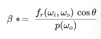
다음으로, BRDF 함수가 달라지면 위 수식에서 $\beta$라는 최종 에너지량을 계산하는 함수에서 $f_r$도 달라지고 $p$도 달라지게 된다.
- 반구 범위 샘플링 시, pdf의 분포에 따라 방향이 샘플링되기 때문에 BRDF 샘플링 방법에 영향을 받는다.
- 에너지 양을 계산하는 함수 자체가 달라지고 pdf 분포도 달라지므로 최종적인 계산식에도 영향을 준다.
최종적으로 아래 코드처럼, 바운스한 광선이 광원에 닿아서 cotribute의 값이 0보다 커지게 되어 화면에 영향을 줄 수 있는 값이 되어 시각적으로 표현되는 것이다.
        if (is_emissive(obj)) {
            if (depth == 0 || lastSpecular) {
                // depth==0 -> camera가 직접 본 조명은 direct에,
                // specular chain 후 본 조명은 indirect에 누적
                Vec3 contrib = mul(beta, obj.e);
                if (depth == 0) result.direct += contrib;
                else            result.indirect += contrib;
            }
            break; // 광원에 닿았으면 종료 (불필요한 추가 샘플 방지)
        }
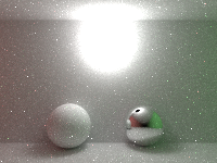
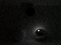
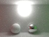
위부터 순서대로 Direct→Indirect→(Direct + Indirect)의 결과 이미지이다.
전체 코드
// --------------------- Path Tracing w/ NEE ---------------------
RadianceResult radiance(Ray ray, RNG& rng, int maxDepth) {
    RadianceResult result{ Vec3(0.0), Vec3(0.0) };
    Vec3 beta(1.0);         // path throughput
    bool lastSpecular = false;

    for (int depth = 0; depth < maxDepth; ++depth) {
        double t; int id;
        if (!intersect_scene(ray, t, id)) break;

        const Sphere& obj = scene[id];
        Vec3 hit = ray.o + ray.d * t;
        Vec3 n = normalize(hit - obj.p);
        Vec3 nl = (dot(n, ray.d) < 0) ? n : n * -1.0;

        // ----- Add emission (only if directly visible or after specular events) -----
        if (is_emissive(obj)) {
            if (depth == 0 || lastSpecular) {
                // depth==0 -> camera가 직접 본 조명은 direct에,
                // specular chain 후 본 조명은 indirect에 누적
                Vec3 contrib = mul(beta, obj.e);
                if (depth == 0) result.direct += contrib;
                else            result.indirect += contrib;
            }
            break; // 광원에 닿았으면 종료 (불필요한 추가 샘플 방지)
        }

        // ----- Russian roulette after a few bounces -----
        if (depth > 3) {
            double q = std::max(0.05, std::min(0.9, std::max({ obj.albedo.x, obj.albedo.y, obj.albedo.z })));
            if (rng.uniform() >= q) break;
            beta = beta / q;
        }

        // ----- Specular material -----
        if (obj.mat == SPECULAR) {
            Vec3 refl = ray.d - n * (2.0 * dot(n, ray.d));
            ray = Ray(hit + nl * 1e-4, normalize(refl));
            beta *= obj.albedo;      // delta BRDF: f*cos/pdf = albedo
            lastSpecular = true;
            continue;
        }

        // ----- NEE: Direct lighting from sampled light -----
        if (!lights.empty()) {
            // 1) pick a random light uniformly
            std::uniform_int_distribution<size_t> pick(0, lights.size() - 1);
            size_t li = pick(rng.gen);
            const Sphere* lightPtr = lights[li];
            const Sphere& light = *lightPtr;

            // 2) 라이트 표면 균등 샘플
            double r1 = 2.0 * PI * rng.uniform();
            double z = 1.0 - 2.0 * rng.uniform();            // in [-1,1]
            double rxy = std::sqrt(std::max(0.0, 1.0 - z * z));
            // Light의 normal vector를 균등 샘플링을 통해 추출한다.
            Vec3 light_n = normalize(Vec3(rxy * std::cos(r1), rxy * std::sin(r1), z));
            Vec3 x_light = light.p + light_n * light.r;

            // 3) 방향/거리/코사인
            Vec3 toL = x_light - hit;
            double d2 = dot(toL, toL);
            double d = std::sqrt(d2);
            Vec3  wi = toL / d;
            double cos_i = std::max(0.0, dot(nl, wi));   // 표면쪽
            double cos_l = std::max(0.0, dot(light_n, -1.0 * wi)); // 라이트쪽

            // 4) 가시성: 첫 교차가 선택한 라이트면 통과 (거리비교 X)
            bool occluded = false;
            {
                Ray shadow_ray(hit + nl * 1e-4, wi);
                double tS; int idS;
                if (intersect_scene(shadow_ray, tS, idS)) {
                    const Sphere* firstHit = &scene[idS];
                    if(tS < (d - std::max(1e-4, 1e-3 * d))) occluded = true;
                    occluded = (firstHit != lightPtr);
                }
            }

            // 5) 기여
            if (!occluded && cos_i > 0.0 && cos_l > 0.0) {
                // PPT의 pdf_solid_angle
                double area = 4.0 * PI * light.r * light.r;
                double pdf_omega = (d2) / (cos_l * area);           // 표면균등 샘플의 고체각 pdf
                pdf_omega /= static_cast<double>(lights.size());    // 라이트 균등 선택까지 포함

                Vec3 f = obj.albedo * (1.0 / PI);                  // Lambert f
                Vec3 Li = light.e;

                // PPT식: L += f * Li * cos_i / pdf_omega
                Vec3 contrib = mul(beta, mul(f, Li)) * (cos_i / std::max(pdf_omega, 1e-12));
                result.direct += contrib;
            }
        }

        // ----- Indirect bounce (cosine-weighted hemisphere) -----
        double r1 = 2.0 * PI * rng.uniform();
        double r2 = rng.uniform();
        double r2s = std::sqrt(r2);

        Vec3 u = normalize(cross((std::fabs(nl.x) > 0.1 ? Vec3(0, 1, 0) : Vec3(1, 0, 0)), nl));
        Vec3 v = cross(nl, u);
        Vec3 d = normalize(u * (std::cos(r1) * r2s) + v * (std::sin(r1) * r2s) + nl * std::sqrt(1.0 - r2));

        ray = Ray(hit + nl * 1e-4, d);
        beta *= obj.albedo;  // for cosine-weighted sampling of Lambertian: f*cos/pdf = albedo
        lastSpecular = false;
    }
    return result;
}
« Monte Carlo 방법의 수학적 기초
How the direction are sampled from BRDF? »