How the direction are sampled from BRDF?
2025/11/12 written. 2025/11/26 updated.
Reference
pbrt v3, https://www.pbrt.org/
Background
In advance, We know Transforming between distributions. In describing the inversion method, pbrt introduce this chapter.
We are given random variable $X_i$ from PDF $p_x(x)$. If we compute $Y_i = y(X_i)$, we would like to find the distribution of the new random variable $Y_i$. But, We cannot understand this kind of transformation for multidimensional distribution functions.
Suppose $y$ being one-to-one mapped on $x$, which implies that,
\[\begin{align}Pr(Y \leq y(x))=Pr(X\leq x) \rightarrow P_y(y)=P_y(y(x))=P_x(x).\end{align}\]Note that $P_x(x)$ means probability value of CDF. So, $P_x(x)$ is made from $p_x(x)$. CDFs leads to the relationship between their PDFs. Since
\[\begin{align}p_x(x)=\frac{d}{dx}P_x(x) \end{align}\], we take the derivative of $P_y(y(x))=P_x(x)$. The right-hand side is $\frac{d}{dx}P_x(x) = p_x(x)$ and the left-hand side is $\frac{d}{dy}P_y(y(x))=\frac{dP_y(y)}{dy}\cdot\frac{dy}{dx}.$
Therefore,
\[\begin{align} p_y(y) \cdot \frac{dy}{dx} = p_x(x) \rightarrow p_y(y) = (\frac{dy}{dx})^{-1} p_x(x). \end{align}\]For example, We have $X$ drown from $p_x(x)$ and want to compute $Y$ from $p_y(y)$. Thus, we use that formula to compute $Y$. We know PDF $p_y(y),$ but we want to know $Y$ sampled from $p_y(y)$.
However, it’s too hard. It’s different from drawing sample from distribution and knowing distribution. So, a sample $Y$ (from the desired distribution $p_y$) is obtained by transforming a sample $X$ drawn from a simple distribution $p_x$(like uniformly distribution). We generalize this formula, which is
\[\begin{align} y(x)=P_y^{-1}(P_x(x)). \end{align}\]Let $y(x)=y=T(x)$, the densities are related by
\[\begin{align} p_y(y)=p_y(T(x))=\frac{p_x(x)}{J_T(x)}. \end{align}\]$J_T$ is the absolute value of determinant of $T$.
Spherical coordinates
\(\begin{align}
&x=rsin\theta cos\phi \\
&y=rsin\theta sin\phi \\
&z=rcos\theta
\end{align}\)
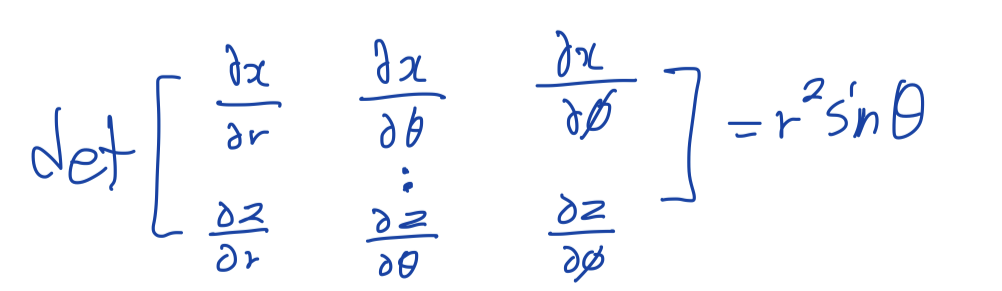 The $J_T=r^2 sin \theta$, the density function is $p(r, \theta, \phi)=r^2\cdot sin\theta \cdot p(x, y, z)$. This transformation means to represent directions as points $(x, y, z)$ on unit sphere in Cartesian coordinates. Solid angle $\Omega$ is defined as the area of a set of points on unit sphere. On unit sphere($r=1$), $d\omega$ over a solid angle can be derived
since $J_T$ is the transformation function that defines the relationship between two coordinate spaces. So, if we knew a density function CDF $Pr(\omega \in \Omega)$ is $\int_\Omega p(\omega) d\omega$, the PDF $p$ with respect to $\theta$ and $\phi$ is
\[\begin{align} p(\theta, \phi) d\theta d\phi = p(\omega) d\omega \\ p(\theta, \phi)=sin \theta p(\omega) \end{align}\]Note that the probability for (very small) orientation region must be the same, whether the orientation is expressed in $\omega$ or in $(\theta, \phi)$. Because, they refer to the same thing in each space. Therefore, $J_T$ is $sin\theta$ on unit sphere from solid angle to polar coordinate.
Uniformly! Sampling A Hemisphere
For example, we consider the task of sampling a direction on the hemisphere uniformly with respect to solid angle. We have a goal that is to use uniformly sampling for sampling $Y$ is drawn from the distribution PDF $p(y)$. Otherwise, the random number $(u, v)$ is converted to angle $(\theta, \phi)$ following the distribution $p(\theta, \phi)$ we want. In this example, $p(\theta, \phi)$ means the hemisphere space.
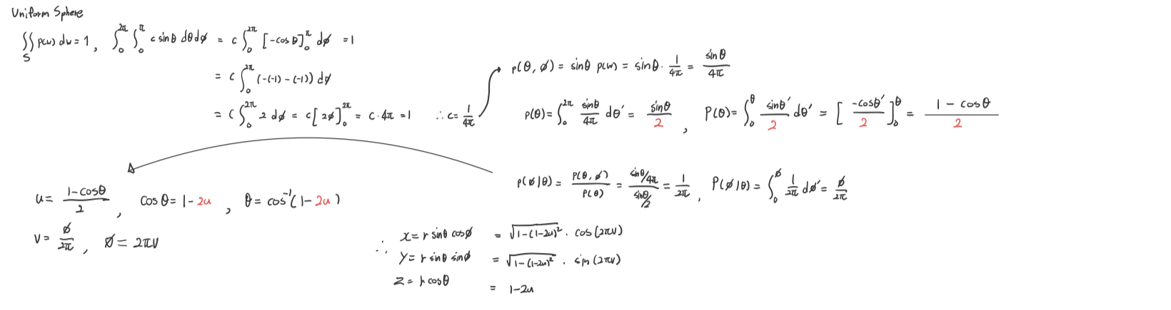
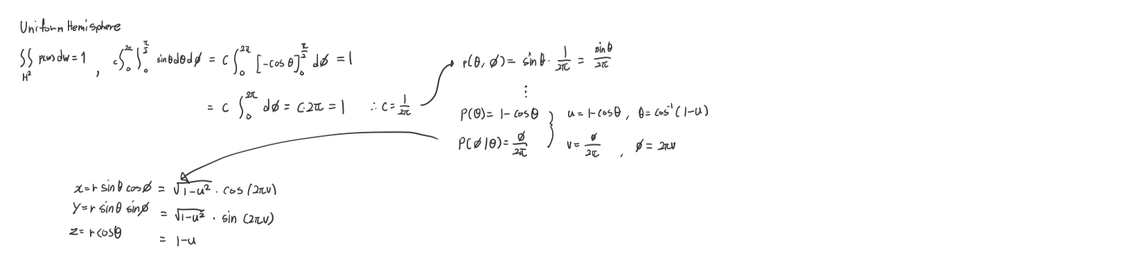
First, we have to know what is $p(\omega)$ defined on hemisphere space. The integral of the PDF $p(\omega)$ over its entire domain is 1. Note that a uniform distribution means that the density function is constant $c$. (we said $d \omega= sin\theta d\theta d\phi$)
\[\begin{align} \int_{\mathcal{H}^2} p(\omega) d\omega =1 \rightarrow c\int_{\mathcal{H}^2} d\omega =1 \rightarrow c = \frac{1}{2\pi} \end{align}\]We have learned $p(\theta, \phi) = sin\theta \ p(\omega)$. So, $p(\theta, \phi) = \frac{sin\theta}{2\pi}$. Therefore,
\[\begin{align} p(\theta)=\int^{2\pi}_{0} p(\theta, \phi) d\phi = sin \theta, \ P(\theta)=\int^\theta_0 sin \theta' d\theta'=1-cos\theta \end{align}\] \[\begin{align} p(\phi | \theta)= \frac{p(\theta, \phi)}{p(\theta)}=\frac{1}{2\pi},\ P(\phi|\theta)=\int^\theta_0 \frac{1}{2\pi}d\phi'=\frac{\phi}{2\pi} \end{align}\]We said a sample $Y$ (from the desired distribution $p_y$) is obtained by transforming a sample $X$ drawn from a simple distribution $p_x$(like uniformly distribution). That is, $u = P(\theta) = 1-cos\theta$ and \(v = P(\phi \| \theta) = \frac{\phi}{2\pi}\) can derive theta and phi, which is
Finally, we have obtained theta and phi for uniformly hemisphere sampling from our uniform random variables. Now, we can derive the Cartesian coordinates (x, y, z) simply by plugging these angles into the spherical coordinate conversion formulas.
Cosine-Weighted! Hemisphere Sampling
If we suppose that we do not want uniformly hemisphere sampling, we may want hemisphere sampling to be more centered. So, we can define $p(\omega)\propto cos\theta$. It’s different from constant we explained.
Expansion procedure is the same. First, We find $c$.
\[\begin{align} \int_{\mathcal{H}^2} p(\omega) d\omega =1 \rightarrow \int_{\mathcal{H}^2}c\cdot cos\theta \ d\omega =1 \rightarrow c\int^{2\pi}_{0} \int^{\frac{\pi}{2}}_0 cos\theta sin\theta \ d\theta d\phi =1 \rightarrow c =\frac{1}{\pi} \end{align}\]That’s why we know that cosine-weighted hemisphere have PDF $p(\omega)=\frac{1}{\pi}cos\theta$. Therefore, $p(\theta, \phi)=sin\theta \ \frac{1}{\pi}cos\theta$.
Second, we compute $p(\theta)$ and $p(\theta, \phi)$. And then we know theta and phi for cosine-weighted hemisphere sampling using inversion transformation.
Other approach exist about cosine-weighted hemisphere sampling. We can use unit disk. That means 2D disk can be projected to 3D hemisphere.
In advance, we know how to sample from uniformly unit disk.
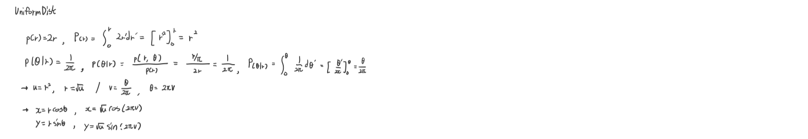
\[\begin{align} c\int\int_D p(x, y) dxdy = 1 \rightarrow c\int^{2\pi}_0 \int^1_0 rdrd\theta = 1 \rightarrow p(\omega) = \frac{1}{\pi} \\ p(r, \theta) = r \cdot p(x, y) = \frac{r}{\pi} \\ p(r) = \int^{2\pi}_0 p(r, \theta) d\theta = 2r \\ p(\theta | r) = \frac{p(r, \theta)}{p(r)} = \frac{1}{2\pi} \end{align}\]$p(r, \theta) = r \cdot p(x, y), \ dxdy = r dr d\theta$. As repeating we explained procedure, we can obtain $r=\sqrt{u}$ and $\theta = 2\pi v$. Therefore, $x=\sqrt{u} sin(2\pi v)$ and $y=\sqrt{u} \cos(2\pi v)$. According to Malley’s Method,
\[\begin{align} x^2+y^2+z^2 = 1 \rightarrow z= \sqrt{1-x^2-y^2} \end{align}\]we can see only two coordinates is used to compute $z$.
Note that $p(\omega)$ is the direction of samples, which we want to pick up a certain shape. That’s why Uniformly sampling has $p(\omega) = c$. Because we want to sample uniformly for all direction. Therefore, cosine-weighted sampling has $p(\omega) \propto cos\theta$.
We must know the ray tracer code want to know $p(\omega)$. Because $p(\omega)$ means probability of sampled direction from PDF. The ray tracer will use $p(\omega)$ as a denominator of Monte Carlo Estimation.
Apply Sampling Algorithm in practice with NORI
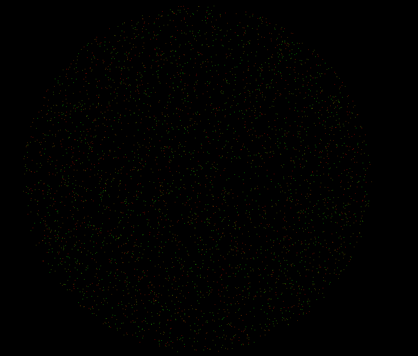
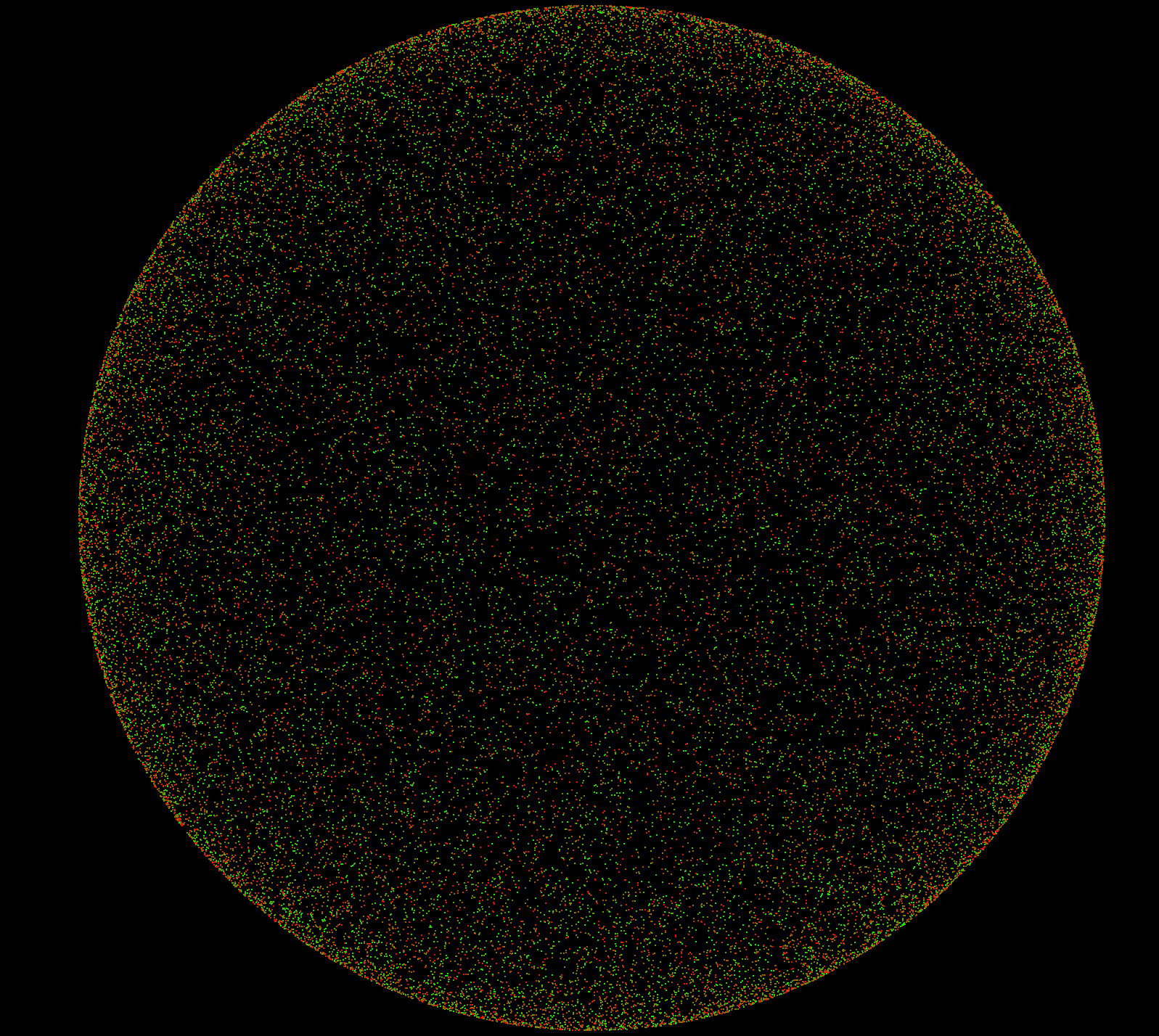
1. UniformDisk
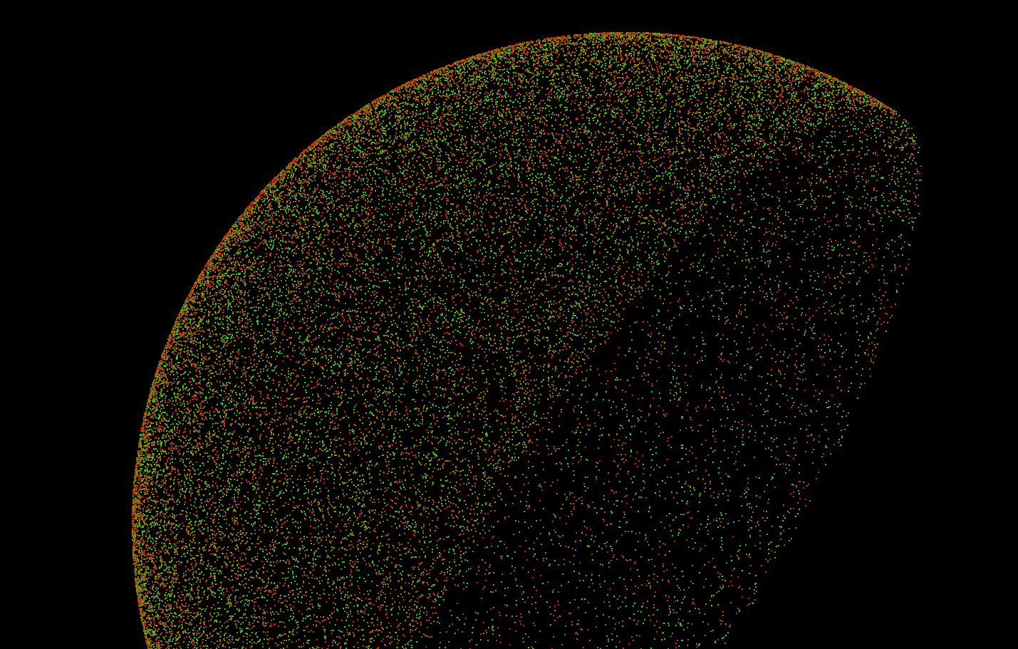
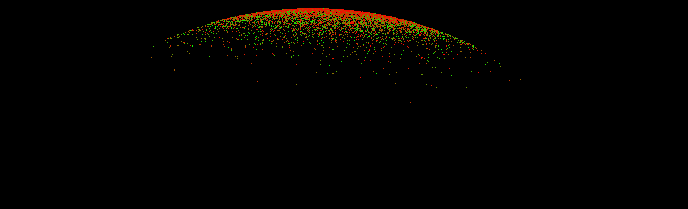
2. UniformSphere
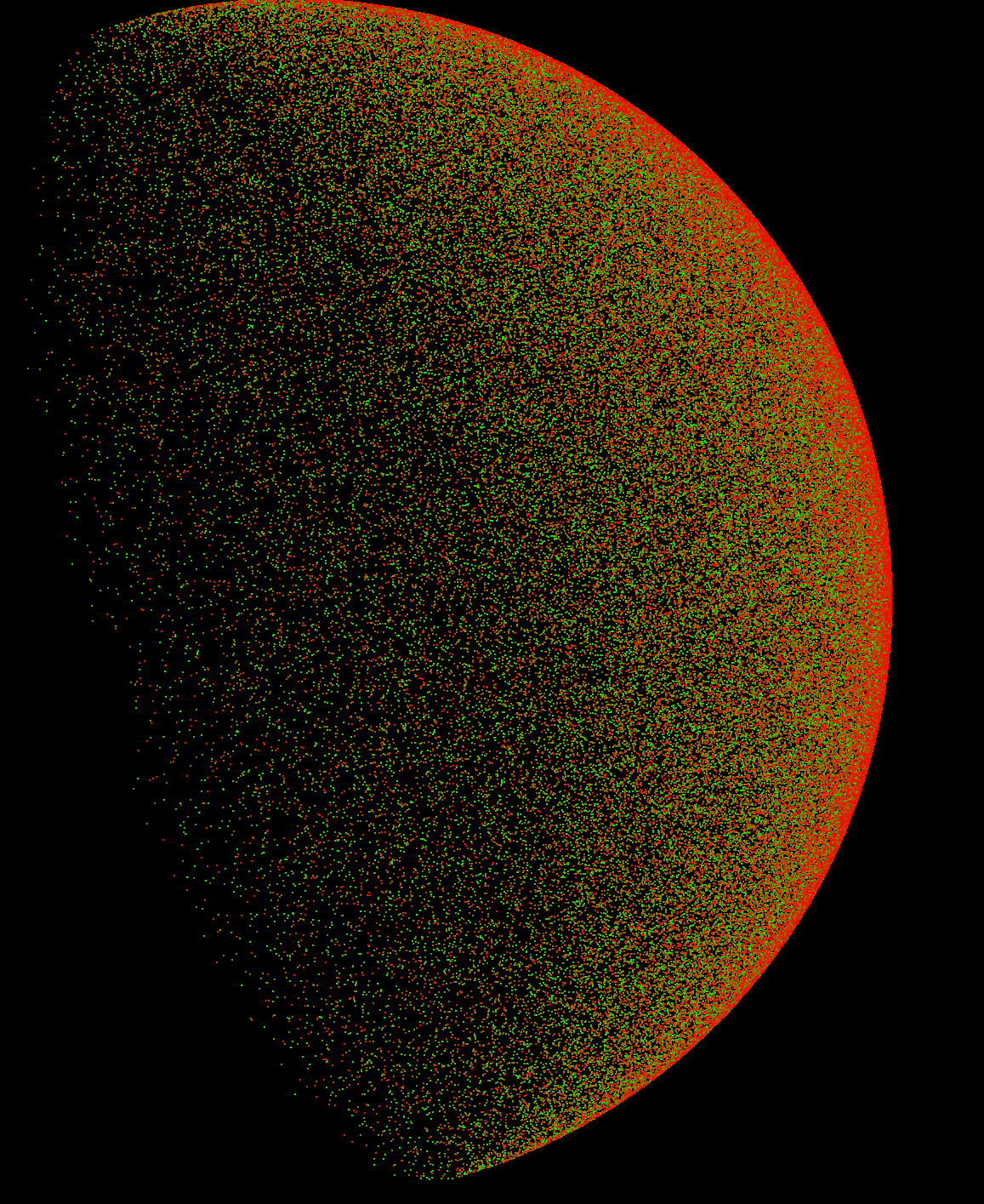
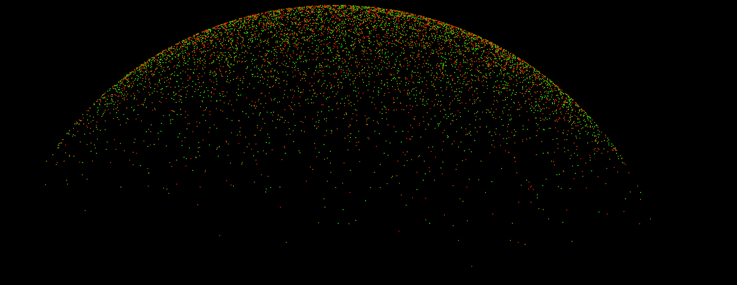
3. UniformHemisphere
4. Cosine-weighted Hemisphere

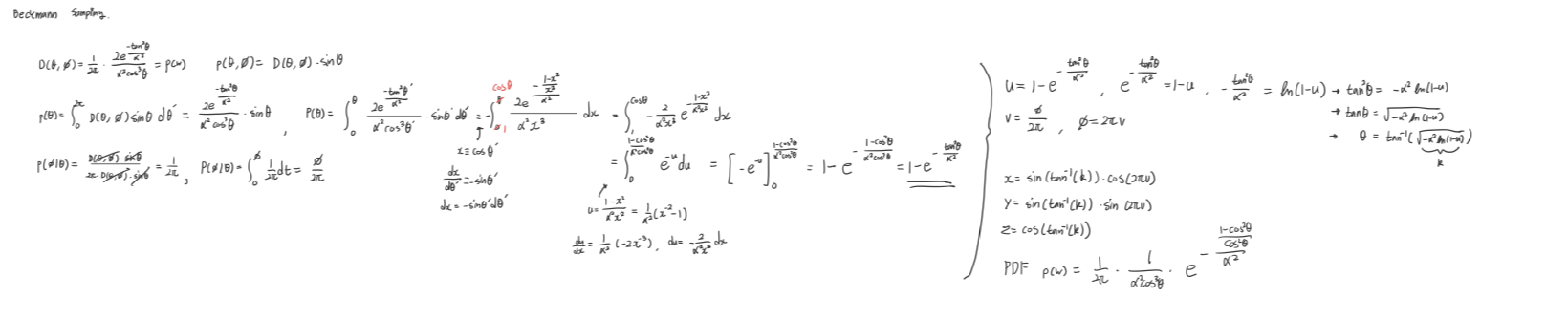
5. Beckmann Function
« Naive Path Tracing: From Formula to Code
Acceleration Data Structures with NORI »