2025/11/24 written. 2025/11/30 updated.

Reference

• pbrt v3, https://www.pbrt.org/
• Nori Renderer.

Whitted Ray tracing

This method is designed to simulate refraction and reflection. Suppose some object has perfectly reflection, such as mirror. So, We can know reflection vector $r$ is computed by

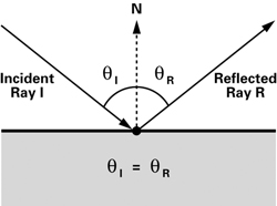
In world coordinates, we just insert value into this formula as it is. However, let us consider local coordinates. We know normal vector is $(0, 0, 1)$ in local coordinates. Therefore, we can compute

Not only dielectric materials(like diamonds, glass, water, …) have perfectly reflection but also has refraction. How we compute dielectric materials that have transparent. The refraction is based on snell's Law and more different than reflection.

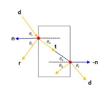
Snell’s law means $n_i sin\theta_i=n_o sin\theta_o$. $n_i$ and $n_o$ are constant ratio of refraction about object(air, glass). That is, $\frac{n_i}{n_o} = \mathfrak{n}(\mathsf{refraction\ ratio})$.

We may define $\textbf{t} = \sin\theta_o \textbf{b}+cos\theta_o(\textbf{-n})$. We wonder that how we define $\textbf{t}$? You can think vector sum.

But, they($\textbf{t},\ \textbf{b}$) are unknown. Hence, We can define $\textbf{b}$ using $\textbf{d} = sin\theta_i \textbf{b} - cos\theta_i (\textbf{n})$. Thus, $\textbf{b} = \frac{\textbf{d} + \textbf{n} cos\theta_i}{sin\theta_i}$ and $\textbf{t} = sin\theta_o (\frac{\textbf{d} + \textbf{n} cos\theta_i}{sin\theta_i}) - cos\theta_o \textbf{n}$. In the above figure, we can found $cos^2 \theta_o$ using $cos^2 \theta_i$. Finally, we know that how we define $\textbf{t}$..!

You may take a question, saying that there’s still a problem $sim\theta_o$. However, if you look at the formula that I described at the Snell’s Law, we can know $sin\theta_o = \frac{n_i}{n_o}sin\theta_i$.

The ray is defined by $R = o + \textbf{t}d$. Thus, we can compute which direction the rays will move in. On the other hand, if you’re going from the inside to the outside, we just change $i$ and $o$. In the code,

if (cosThetaI < 0.0f) { 
	// 1. change n_i and n_o (1.0/1.5 -> 1.5/1.0) 
	std::swap(etaI, etaT); 
	// 2. -wi.dot(n) = cosThetaI -> -wi.dot(-n) = -cosThetaI
	cosThetaI = -cosThetaI; 
}

So far, it’s been an explanation in the world coordinates. Now let us consider the situation in the local coordinates. It’s so simple. Because normal vector is (0, 0, 1). We insert it into $\textbf{t}$.

We can compute $x’$, $y’$, $z’$ in local coordinate.